Month: May 2018

I just published my series on Graph Databases a few hours ago, and have already had lots of hits. I guess people found the topic as interesting as I did! One reader, Jay Pipes, is one of the core developers of the Placement service I mentioned in that series, and probably the most heavily opinionated with regards to using MySQL. He is also a long-time friend. Jay asked some excellent questions at the end of the last post, and I didn’t feel that I could do them justice in the space of a WordPress reply box, so I created this post. Let’s get into it!

1) I note that you’ve combined allocations and inventory into a single object. How would we query for the individual consumers of resources?

The combination was for simplifying the illustration. As you can probably guess, a full Placement model would have Consumer objects that would have a [:CONSUMES] relation to the resource objects. So to illustrate this, I added another script to the GitHub repo: create_consumer.py. Since  relations can have properties too, we’d create an ‘amount’ property that would specify how much of a resource is being consumed by this particular consumption. The query would look something like this:

MATCH (disk:DISK_GB)<-[alloc:CONSUMES]-(con:Consumer)
WITH disk, disk.total - SUM(alloc.amount) AS avail
WHERE avail > 2000
RETURN disk, avail

This would return the disks whose total amount minus the sum of all the consumed amounts, is greater than 2000.

2) How many resources of each type are being consumed by a project or user or consumer? (i.e. usages, aggregated by a grouping mechanism – the thing that SQL does pretty well)

In this respect, it wouldn’t be all that different. Cypher does aggregates, too. Using the data generated by the create_consumer.py script, I can run the following query:

MATCH (con:Consumer)-[alloc:CONSUMES]->(r)
WHERE con.pk = 1
RETURN labels(r)[0] AS resource_class, sum(alloc.amount) AS usage

This query will return:

╒════════════════╤═══════════════════╕
│"resource_class"   │"usage"                │
╞════════════════╪═══════════════════╡
│"MEMORY_MB"        │1024                   │
├────────────────┼───────────────────┤
│"DISK_GB"          │500                    │
├────────────────┼───────────────────┤
│"VCPU"             │2                      │
└────────────────┴───────────────────┘

So as you can see, not a whole lot different than with SQL.

3) How do you ensure that multiple concurrent writers do not over-consume resources on a set of providers? We use a generation on the provider along with an atomic update-where-original-read-generation strategy to protect the placement DB objects. I’m curious how neo4j would allow that kind of operation.

Neo4j is ACID-compliant, and transactions either succeed completely or not at all. So I’m not really sure how much I can add to that. Setting the value of an object is trivial, updating that value is trivial, checking a supplied value with the one stored in the DB is trivial. So it would work identically to how it works in SQL.

In summary, I want to make two points: first, I’m not bashing MySQL. It’s an excellent database that I use extensively myself (well, I use MariaDB, but…). This WordPress site has a MariaDB backend. Second, this started as an attempt to scratch the itch I have felt since we began making Placement more and more complex. I wanted to find out if there was a better way to handle the sort of problems we have, and my previous reading on graph databases came to mind. It was tough to get used to thinking with a graph mindset. It reminded me of when I first started using Go after years of Python: when I tried to write Pythonic code in Go, it was terrible. Once I was able to drop the Python mindset and write Go the way it was designed, things were much, much easier to understand, and the code I wrote was much, much better. The same sort of “letting go” process had to happen before I was able to fully see what can be done with graph databases.

In the previous two posts in this series, I wrote about graph databases in general, and why I think that they are much more suited to modeling the data in the Placement service than relational DBs such as MySQL. In this post I’ll show a few examples of common Placement issues and how they are solved in Neo4j. The code for all of this is in my GitHub repo. I’ll cover the two biggest sources of complexity: Nested Resource Providers and Shared Providers.

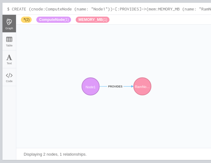
Nested Resource Providers: this refers to the case where one ResourceProvider physically contains one or more other ResourceProvider, and it is this contained provider that is the source of the requested resources. This nesting forms a tree-like structure, and can go arbitrarily deep, although in practice it would be rare to see case where it was more than 4 levels deep. One such case that Placement needs to handle is a compute node containing NUMA nodes. With NUMA, some of the resources, such as disk, can be supplied by the ComputeNode, while others, such as RAM and VFs, come from the NUMA node. The response needs to not only include the selected ComputeNode, but the entire tree of ResourceProviders.

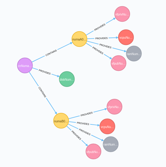
To illustrate this example, I’m going to create 50 plain compute nodes, and 50 that contain 2 NUMA nodes each. The plain computes will provide disk, RAM, VCPU and VFs, while on the NUMA computes, the compute node will only provide the disk; the RAM, VCPU, and VFs are provided by the NUMA node. The script will gradually decrease the amount of available resources by increasing the value assigned to ‘used’ as it runs. To make a script like this, I used the py2neo module; there are several Python wrappers for Neo4j; I chose this because it seemed simplest. The code is in the script named create_nested.py.

Let’s start with an easy one: get all the compute nodes that have at least 2000 MB of RAM:

MATCH (cn:ComputeNode)-[*]->(ram:MEMORY_MB)
WHERE ram.total - ram.used > 2000
RETURN cn, ram

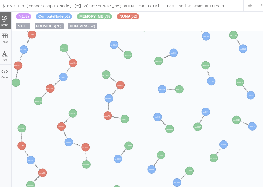
Note that the query returned ComputeNodes (blue) that had the RAM (green) associated through a NUMA node (red) as well as those where the ComputeNode itself supplied the RAM.

You can match any number of filters with a single query. While it is possible to create long, complex queries in Cypher, it is simpler and more idiomatic to use the WITH clause to chain the results of one query with the results of the next:

MATCH p=(cnode:ComputeNode)-[*]->(ram:MEMORY_MB)
WHERE ram.total - ram.used > 4000
WITH p, cnode, ram
MATCH (cnode:ComputeNode)-[*]->(disk:DISK_GB)
WHERE disk.total - disk.used > 2000
RETURN p, cnode, disk, ram

So while this might look like a JOIN or UNION in SQL, it is interpreted by Cypher as a single query, and executed as such. This will return the following. Note that once again there are Compute Nodes both with and without NUMA nodes coming back from the same query.

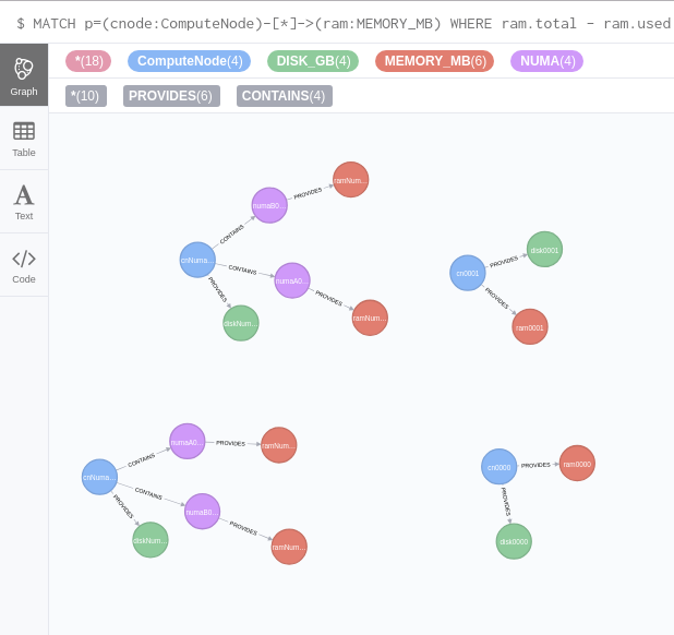
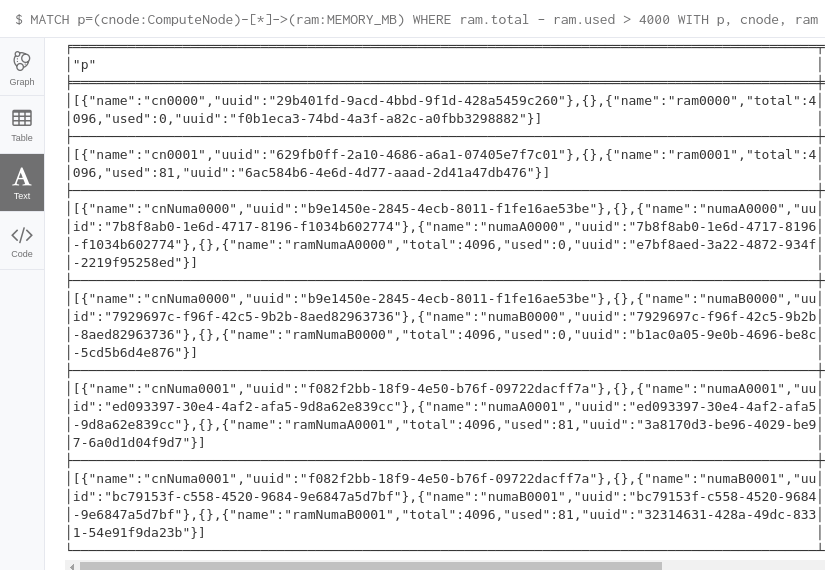
Ok, you’re thinking, this is all very fine, but what am I going to do with a bunch of colored circles and lines? Fear not. This is just the visualization of the returned data. You can also see the results in plain text:

Here it’s even clearer that even though there are only 4 ComputeNodes returned, there are 6 possible solutions, since each of the nodes with NUMA can satisfy the request with either NUMA node. This is returning the entire tree structure, which is what Placement requires for such queries.

When you run the query using py2neo, you get lists of Python dicts for the result:

[{'cnode': {'name': 'cn0000',
            'uuid': '29b401fd-9acd-4bbd-9f1d-428a5459c260'},
  'disk': {'name': 'disk0000',
           'total': 2048,
           'used': 0,
           'uuid': '605c622e-4f9a-4e47-9b34-73fbcba624fa'},
 'ram': {'name': 'ram0000',
         'total': 4096,
         'used': 0,
         'uuid': 'f0b1eca3-74bd-4a3f-a82c-a0fbb3298882'}},
 {'cnode': {'name': 'cn0001',
            'uuid': '629fb0ff-2a10-4686-a6a1-07405e7f7c01'},
  'disk': {'name': 'disk0001',
           'total': 2048,
           'used': 40,
           'uuid': '424414a2-5257-4747-abb5-96c407a2cbaf'},
  'ram': {'name': 'ram0001',
          'total': 4096,
          'used': 81,
          'uuid': '6ac584b6-4e6d-4d77-aaad-2d41a47db476'}},
 {'cnode': {'name': 'cnNuma0000',
            'uuid': 'b9e1450e-2845-4ecb-8011-f1fe16ae53be'},
  'disk': {'name': 'diskNuma0000',
            'total': 2048,
            'used': 0,
            'uuid': '7238e020-d628-4bdb-8549-8baffcf08271'},
  'ram': {'name': 'ramNumaA0000',
          'total': 4096,
          'used': 0,
          'uuid': 'e7bf8aed-3a22-4872-934f-2219f95258ed'}},
 {'cnode': {'name': 'cnNuma0000',
            'uuid': 'b9e1450e-2845-4ecb-8011-f1fe16ae53be'},
  'disk': {'name': 'diskNuma0000',
           'total': 2048,
           'used': 0,
           'uuid': '7238e020-d628-4bdb-8549-8baffcf08271'},
  'ram': {'name': 'ramNumaB0000',
          'total': 4096,
          'used': 0,
          'uuid': 'b1ac0a05-9e0b-4696-be8c-5cd5b6d4e876'}},
 {'cnode': {'name': 'cnNuma0001',
            'uuid': 'f082f2bb-18f9-4e50-b76f-09722dacff7a'},
  'disk': {'name': 'diskNuma0001',
           'total': 2048,
           'used': 40,
           'uuid': '2a7004b8-001c-4244-bf84-0a511f8a3eb1'},
  'ram': {'name': 'ramNumaA0001',
          'total': 4096,
          'used': 81,
          'uuid': '3a8170d3-be96-4029-be97-6a0d1d04f9d7'}},
 {'cnode': {'name': 'cnNuma0001',
            'uuid': 'f082f2bb-18f9-4e50-b76f-09722dacff7a'},
  'disk': {'name': 'diskNuma0001',
           'total': 2048,
           'used': 40,
           'uuid': '2a7004b8-001c-4244-bf84-0a511f8a3eb1'},
  'ram': {'name': 'ramNumaB0001',
          'total': 4096,
          'used': 81,
          'uuid': '32314631-428a-49dc-8331-54e91f9da23b'}}]

 

Let’s look at the other use case that complicates Placement: Shared Providers. The most common usage is when a large disk array is shared among many compute nodes. So to simulate that case, I created a single ComputeNode with local disk storage, and two without. Next I created 2 shared disk providers, one with a much greater capacity than the other. I also created 2  ComputeNodes, neither of which has local disk. The next step is to create an Aggregate that will be used to associate these diskless ComputeNodes with the shared disks. Now it really isn’t necessary to do this in Neo4j; I could simply associate the shared disks directly with the ComputeNodes. With graph databases this intermediate artifact to associate things is redundant, since relationships are first-class entities. But I’m adding this extra layer in order to make it more familiar with those who work with Placement today. The script for that is create_shared.py, and creates a deployment that looks like this:

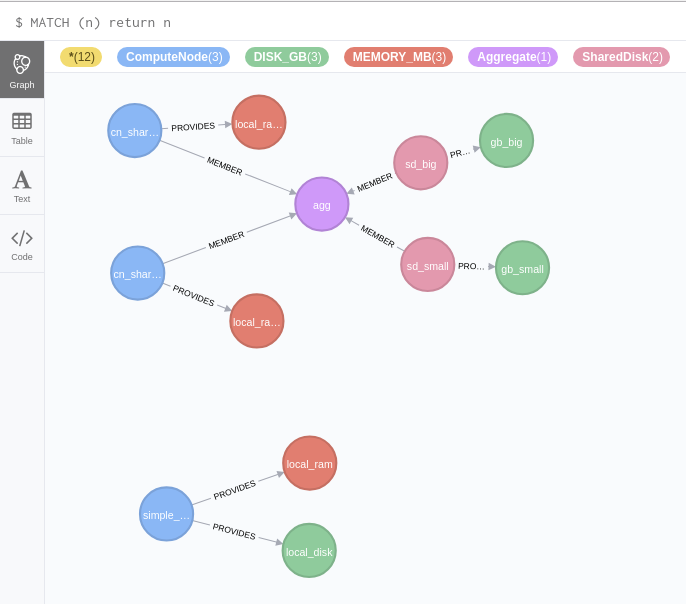
The local disk has 4000GB, the smaller shared disk has 10,000GB, and the larger shared disk has 100,000GB. Let’s run 3 queries, requesting 2,000GB, 8,000GB, and 50,000GB. The code for these queries is in ‘search_shared.py‘, and it looks like this:

MATCH (cnode:ComputeNode)-[*]-(gb:DISK_GB)
WHERE gb.total - gb.used > 50000
RETURN cnode, gb

If you have a sharp eye, you’ll notice something slightly different with this. Prior to this, queries had the format:

(obj)-[relation]->(obj)

In this one, the “arrow” on the right is gone:

(obj)-[relation]-(obj)

Relationships is Neo4j are always defined with a direction (e.g., (Alice)-[:KNOWS]->Bob). But you can query either with or without specifying the direction of the relation. In the shared provider case, there is no directional path between a ComputeNode and a SharedDisk, since they are both related as members of the Aggregate. But they are connected, and the Cypher language allows us to express that we don’t care about the direction of the relationship in some cases. This allows us to use the exact same query to return shared providers as well as local resources.

Finally, let’s combine the two above. In the create_nested_and_shared.py, I took the script for creating a bunch of ComputeNodes, both with and without NUMA, and then added in the shared disks. I associated the first ComputeNode (both with and without NUMA) with that aggregate. The script search_nested_and_shared.py queries nodes for both RAM and increasing amounts of disk. Here’s the query:

MATCH (cnode:ComputeNode)-[*]->(ram:MEMORY_MB)
WHERE ram.total - ram.used > 4000
WITH cnode, ram
MATCH (cnode:ComputeNode)-[*]-(disk:DISK_GB)
WHERE disk.total - disk.used > 2000
RETURN cnode, disk, ram

I ran that query 3 times, each requesting different disk amounts. Here’s the output for requests of 2,000GB, 8,000GB, and 20,000GB  :

Requesting small disk; found 15
[('cn0000', 'gb_small'),
 ('cnNuma0000', 'gb_small'),
 ('cnNuma0000', 'gb_small'),
 ('cn0000', 'gb_big'),
 ('cnNuma0000', 'gb_big'),
 ('cnNuma0000', 'gb_big'),
 ('cn0000', 'disk0000'),
 ('cnNuma0000', 'disk0000'),
 ('cnNuma0000', 'disk0000'),
 ('cn0001', 'disk0001'),
 ('cnNuma0000', 'diskNuma0000'),
 ('cnNuma0000', 'diskNuma0000'),
 ('cn0000', 'diskNuma0000'),
 ('cnNuma0001', 'diskNuma0001'),
 ('cnNuma0001', 'diskNuma0001')]

Requesting medium disk; found 6
[('cn0000', 'gb_small'),
 ('cnNuma0000', 'gb_small'),
 ('cnNuma0000', 'gb_small'),
 ('cn0000', 'gb_big'),
 ('cnNuma0000', 'gb_big'),
 ('cnNuma0000', 'gb_big')]

Requesting large disk; found 3
[('cn0000', 'gb_big'),
 ('cnNuma0000', 'gb_big'),
 ('cnNuma0000', 'gb_big')]

Note that the above was a single query that was identical in structure to the nested-only and shared-only queries. In other words, there was no complex SQL required, no joins, no auxiliary tables, no client-side combination of separate result sets – in other words, no heroic SQL-fu needed. The reason is that graph databases fit the problems of Placement much, much better than traditional relational DBs.

Performance: I suppose that without mentioning performance for these queries, it’s all pointless. I mean, what’s the good of simplified code if it takes forever to run? Well, if you notice, at the top of the create_nested.py script there is a constant NODE_COUNT. I ran my tests with the default setting of 50, which would simulate a deployment of 100 total servers (50 plain, 50 with NUMA). I have this running on a DigitalOcean VM with 2GB RAM, 30GB disk, and 1 VCPU.  When I ran the following query, which is the same one I ran earlier in this post, I got these results:

MATCH p=(cnode:ComputeNode)-[*]->(ram:MEMORY_MB)
WHERE ram.total - ram.used > 4000
WITH p, cnode, ram
MATCH (cnode:ComputeNode)-[*]->(disk:DISK_GB)
WHERE disk.total - disk.used > 2000
RETURN p, cnode, disk, ram

Returned: 78 records
Time: 4ms

OK, that’s wonderful. Now what if we upped that to 1,000 nodes each, or 2,000 total nodes. That’s a pretty good-sized cloud, and running the same query I got:

Returned: 1536 records
Time: 169ms

Not too bad! I couldn’t resist, and increased it to 10,000 nodes each, or 20,000 nodes total! First, please note that the script to create these nodes is terribly inefficient, and creating 20,000 nodes with all their related objects took over an hour. But once the data was there, running the same script returned:

Returned: 15354 records
Time: 831ms

So, even though I haven’t even created a single index, the performance is nothing to worry about.

Summary: Now I know that I didn’t touch Traits, Allocations, Inventory, etc., as I wanted this to be a simple introduction to the concepts of graph databases, and not create a drop-in replacement for the current Placement service. And while I don’t expect the OpenStack Placement team to ever consider anything other than MySQL, I hope you come away from this series at least a little intrigued, and take the time when starting a project to explore alternatives to what you’ve used before. Something that works well in one problem domain doesn’t necessarily work well in others. But when all you have is a hammer, every computing problem looks like a nail to you.