Graph Database Basics

It is not my intent here to create a full tutorial on using graph databases; I just want to convey enough understanding so that you might see why they are a better fit for placement than a relational DB.

The most basic thing to understand is that your whiteboard design is your database design. Here’s what I mean by that:

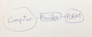
This is the general form of the CREATE statement in Neo4j’s declarative language Cypher:

CREATE (obj1)-[relates_to]->(obj2)

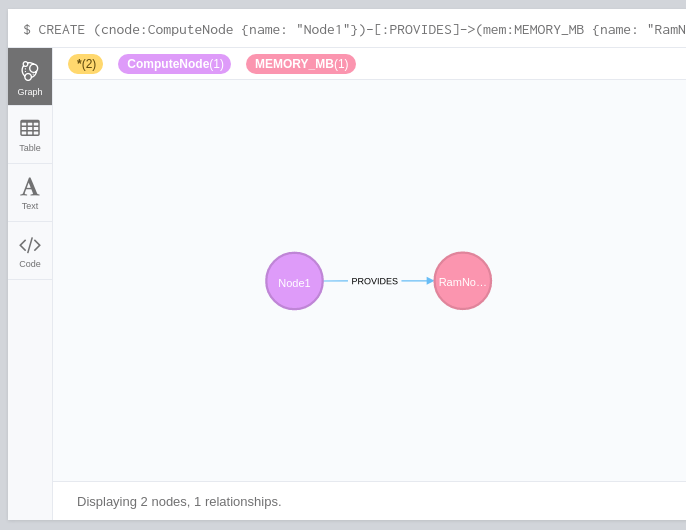
And here is the specific code for creating that in Cypher:

CREATE (cnode:ComputeNode)-[:PROVIDES]->(mem:MEMORY_MB {
    total: 10000, used: 2000})
RETURN cnode, mem

Note that the syntax is close to ASCII diagramming, using parentheses to enclose nodes, square brackets to enclose relationships, dashes to connect them, and arrows to indicate the direction of the relationship. Also note that nodes and relationships can have properties; here I gave the memory a ‘total’ of 10,000, and a ‘used’ value of 2000. These can be used to filter results to only those that have the necessary amounts. I used the Placement standard resource class ‘MEMORY_MB’ for the RAM to make it more familiar.

Neo4j comes with a browser that lets you visualize your data. So when I ran the above code in the browser, I get this back:

Ok, I guess at this point it seems almost toy-like. So here’s something a bit more interesting:

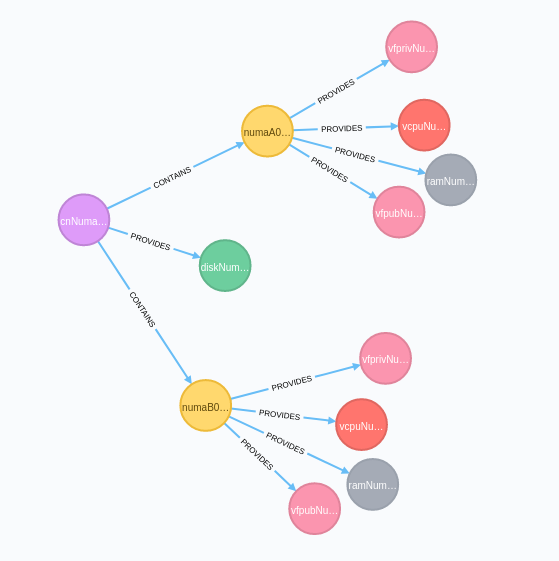
This is a compute node (purple) that provides disk (green), and contains two NUMA nodes (yellow), each of which provides VCPU (orange), RAM (grey), and VFs (pink). The model as stored in the DB matches the real world, and doesn’t require expensive JOINs to retrieve.

And finally (just to show off a little),  I created 500 compute nodes and associated them with aggregates. In Nova/Placement lingo, an ‘aggregate’ is a way to associate things that have something in common. Here’s what one such model looks like:

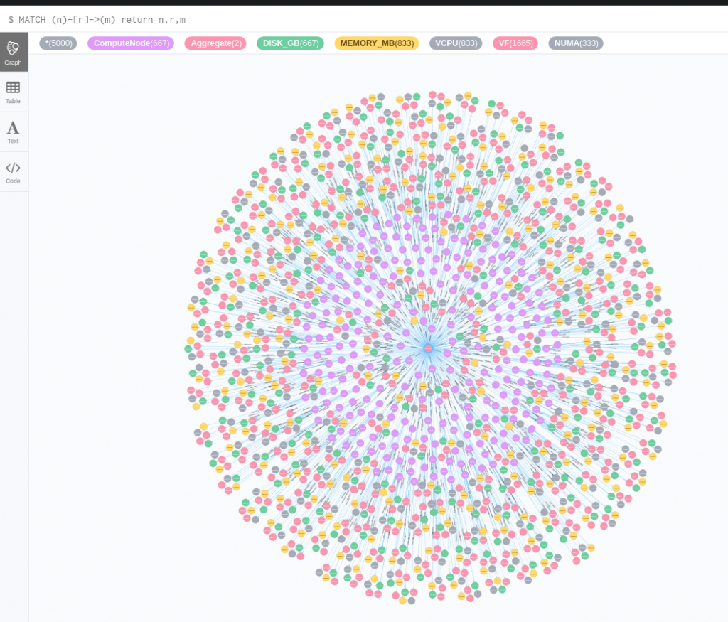
The pink dot in the center is an aggregate, with purple compute nodes attached to it, and attached to those compute nodes are green disks, yellow memory, grey VCPU, and red VFs. And though they are faint, the lines connecting those things are the key to why this works so well: you can traverse these relationships in any direction in a single query– no joins required. I’ll give some specific examples of querying nested and shared resources in the next post in this series.